45 format data labels excel 2016
How to Print Labels from Excel - Lifewire Select Mailings > Write & Insert Fields > Update Labels . Once you have the Excel spreadsheet and the Word document set up, you can merge the information and print your labels. Click Finish & Merge in the Finish group on the Mailings tab. Click Edit Individual Documents to preview how your printed labels will appear. Select All > OK . Excel 2010: How to format ALL data point labels SIMULTANEOUSLY If you want to format all data labels for more than one series, here is one example of a VBA solution: Code: Sub x () Dim objSeries As Series With ActiveChart For Each objSeries In .SeriesCollection With objSeries.Format.Line .Transparency = 0 .Weight = 0.75 .ForeColor.RGB = 0 End With Next End With End Sub. B.
Excel 2016: Formatting Cells - GCFGlobal.org Click the Challenge worksheet tab in the bottom-left of the workbook. Change the cell style in cells A2:H2 to Accent 3. Change the font size of row 1 to 36 and the font size for the rest of the rows to 18. Bold and underline the text in row 2. Change the font of row 1 to a font of your choice.
Format data labels excel 2016
Excel Barcode Generator Add-in: Create Barcodes in Excel 2019/2016… Create 30+ barcodes into Microsoft Office Excel Spreadsheet with this Barcode Generator for Excel Add-in. No Barcode Font, Excel Macro, VBA, ActiveX control to install. Completely integrate into Microsoft Office Excel 2019, 2016, 2013, 2010 and 2007; Easy to convert text to barcode image, without any VBA, barcode font, Excel macro, formula required How to Print Labels from Excel - Lifewire Apr 05, 2022 · How to Print Labels From Excel . You can print mailing labels from Excel in a matter of minutes using the mail merge feature in Word. With neat columns and rows, sorting abilities, and data entry features, Excel might be the perfect application for entering and storing information like contact lists.Once you have created a detailed list, you can use it with other … Excel 2016 Tutorial Formatting Data Labels Microsoft Training ... - YouTube FREE Course! Click: about Formatting Data Labels in Microsoft Excel at . A clip from Mastering Excel M...
Format data labels excel 2016. Excel tutorial: How to use data labels Generally, the easiest way to show data labels to use the chart elements menu. When you check the box, you'll see data labels appear in the chart. If you have more than one data series, you can select a series first, then turn on data labels for that series only. You can even select a single bar, and show just one data label. Format Data Labels Vertically using Pareto in Excel 2016 Re: Format Data Labels Vertically using Pareto in Excel 2016. Try this: Right-click on one of the data labels > Format Data Labels > Size & Properties > Alignment > Text direction: Stacked. Register To Reply. 10-03-2017, 01:19 PM #3. 1gambit. Registered User. Excel 2016: "Value from Cells" box under Format Data Labels Missing 1. The screenshot about the issue. 2. The Office version screenshot via File > Account > Product Information. We will check whether the issue can be reproduced in a specific version. To protect your privacy, please help us mask email address like below: Thanks, Rena ----------------------- * Beware of scammers posting fake support numbers here. Excel Charts: Creating Custom Data Labels - YouTube In this video I'll show you how to add data labels to a chart in Excel and then change the range that the data labels are linked to. This video covers both W...
How to Create Mailing Labels in Excel - Excelchat Step 1 - Prepare Address list for making labels in Excel First, we will enter the headings for our list in the manner as seen below. First Name Last Name Street Address City State ZIP Code Figure 2 - Headers for mail merge Tip: Rather than create a single name column, split into small pieces for title, first name, middle name, last name. Change the format of data labels in a chart To get there, after adding your data labels, select the data label to format, and then click Chart Elements > Data Labels > More Options. To go to the appropriate area, click one of the four icons ( Fill & Line , Effects , Size & Properties ( Layout & Properties in Outlook or Word), or Label Options ) shown here. How to Format Excel Pivot Table - Contextures Excel Tips Jun 22, 2022 · Copy a Custom Style in Excel 2016 or Later. In Excel 2016, the custom pivot table style is not copied, if you use the above technique to copy and paste a pivot table. I found a different way to copy the custom style, and this method also works in Excel 2013. In Excel 2016, follow these steps to copy a custom style into a different workbook: How to format axis labels as thousands/millions in Excel? 1. Right click at the axis you want to format its labels as thousands/millions, select Format Axis in the context menu. 2. In the Format Axis dialog/pane, click Number tab, then in the Category list box, select Custom, and type [>999999] #,,"M";#,"K" into Format Code text box, and click Add button to add it to Type list. See screenshot: 3.
How to hide zero data labels in chart in Excel? - ExtendOffice If you want to hide zero data labels in chart, please do as follow: 1. Right click at one of the data labels, and select Format Data Labels from the context menu. See screenshot: 2. In the Format Data Labels dialog, Click Number in left pane, then select Custom from the Category list box, and type #"" into the Format Code text box, and click Add button to add it to Type list box. Format Data Labels in Excel- Instructions - TeachUcomp, Inc. Nov 14, 2019 · Alternatively, you can right-click the desired set of data labels to format within the chart. Then select the “Format Data Labels…” command from the pop-up menu that appears to format data labels in Excel. Using either method then displays the “Format Data Labels” task pane at the right side of the screen. Format Data Labels in Excel ... How to Add Total Data Labels to the Excel Stacked Bar Chart Apr 03, 2013 · Step 4: Right click your new line chart and select “Add Data Labels” Step 5: Right click your new data labels and format them so that their label position is “Above”; also make the labels bold and increase the font size. Step 6: Right click the line, select “Format Data Series”; in the Line Color menu, select “No line” Edit titles or data labels in a chart - support.microsoft.com The first click selects the data labels for the whole data series, and the second click selects the individual data label. Right-click the data label, and then click Format Data Label or Format Data Labels. Click Label Options if it's not selected, and then select the Reset Label Text check box. Top of Page
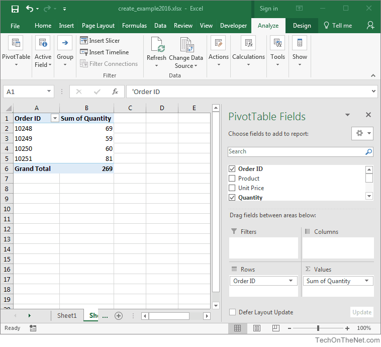
MS Excel 2016: How to Create a Pivot Table
excel - Change format of all data labels of a single series at once ... A workaround (found prior to #1): A very poor solution, but which possibly saves quite a few keystrokes/mouse clicks in many cases. Select the whole chart, and change the font size in the ribbon. It will change all text. Then recover the font size of all other text but the data labels.
November 2018
How to Change Excel Chart Data Labels to Custom Values? May 05, 2010 · Now, click on any data label. This will select “all” data labels. Now click once again. At this point excel will select only one data label. Go to Formula bar, press = and point to the cell where the data label for that chart data point is defined. Repeat the process for all other data labels, one after another. See the screencast.

T-Account Template | How to Excel
Formatting in Excel (Examples) | How to Format Data in Excel? Now we will do data formatting in excel and will make this data in a presentable format. First, select the header field and make it bold. Select the whole data and choose the "All Border option" under the border. Now select the header field and make the thick border by selecting the "Thick box border" under the border.
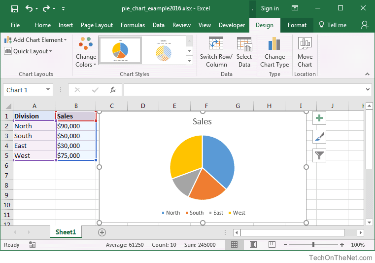
MS Office Suit Expert : MS Excel 2016: How to Create a Pie Chart
Add and format a chart legend - support.microsoft.com Click the chart, and then click the Chart Design tab. Click Add Chart Element > Legend. To change the position of the legend, choose Right, Top, Left, or Bottom. To change the format of the legend, click More Legend Options, and then make the format changes that you want. Depending on the chart type, some options may not be available.
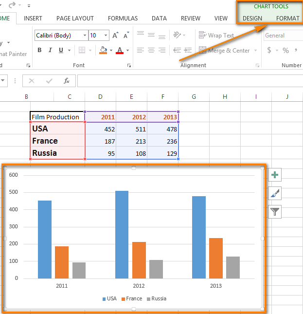
How to add titles to charts in Excel 2016 - 2010 in a minute.
Values From Cell: Missing Data Labels Option in Excel 2016? (Mac) Conshohocken, PA. MS-Off Ver. Office 2016. Posts. 2. Values From Cell: Missing Data Labels Option in Excel 2016? (Mac) I'm trying to format an X Y scatter chart in Excel 2016 (Mac) and I am not seeing an option to include a Value From Cell in my Label Options. Screen Shot 2017-09-06 at 10.40.10 AM.png.
Post a Comment for "45 format data labels excel 2016"